MARCH 27TH, 2014
At A.N.Lab, we develop various applications based on the image-matching and AR (Augmented Reality) technology.
For example, we have developed applications to detect celebrities’ faces from recorded TV programmes, to do book stocktaking from bookshelf pictures, or to recognize corporate logos on paper printings.

The base technology for these application is image-matching.
Here I would like to introduce certain basics of the technology.
Don’t expect to be able to build commercial-level products just by reading these basics, but at least these will give you an idea of how the technology works.
Matching a pair of images
Please look at the below two images.

You can see that the mountain on the right side of the first image and the mountain on the left side of the second image are actually the same one.
Where does a human look at to determine these two mountains are the same ?
Most of the time, humans look at the shapes and the colors.
The image-matching method simulates this behavior. It uses “feature points” that combine the concepts of shapes and colors.
Feature points essentially describe the shapes and the colors of the images.
By matching these feature points, we can see the similarities between the two images.

There are two main steps in the image-matching process.
A. Extracting feature points from the images.
B. Matching the feature points.
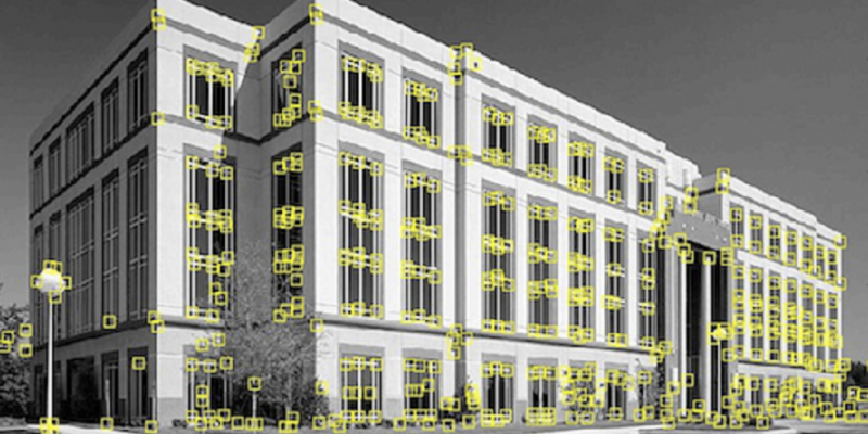
A. Extracting feature points

The shape of the building in this image could be sketched with the positions of the corners (in yellow).
The image-matching method uses these corners as the feature points.
There are algorithms to extract such corner points.
For example, “Harris corner response function” is a well-known one.
Let me skip the mathematical details. Essentially, when we apply the Harris corner function to the below images,

we will get the following results.

Corners would have positive values (red colors).
Lines would have negative values (deep-blue colors).
Flat areas would have values close to zero (light-blue colors).
The local maxima (red points) in this image become the “feature points”.

Note: A local maximum is a point that has the value higher than any neighboring points.
A local maximum is not necessarily the point with the highest value in the whole image.
You can see these local maxima points somehow describe the shape of the object in the image.
Not only corners could be used as feature points
In the below image, not the shapes but the colors actually describe the characteristics of the image better. In this case, we use color areas as the image features.

This method is called “blob detection”.
The areas of the same colors are approximated into circles, and the centers of the circles become the feature points.
B. Matching the feature points
Assume that we have extracted the feature points from the two images.

The more matching feature points are there, the more “similar” the two images are.
The steps for matching feature points are as follows:
———————————
i) Choose two feature points (one from each image) that are “close“, and make them to one pair.
Let the feature point from image A be a, feature point from image B be b.
ii) Compute the transformation from a to b.
The transformation is something like “rotate xx degrees, move to left yy pixels, move upper zz pixels …”.
iii) Apply the above transformation to other feature points in image A. For each of the feature point in image A be transformed, look into image B to see if there is any feature point in B are “close” to the transform point.
The definition of being “close” will be explained later.
———————————

The above example shows the results after the feature points in image A are transformed.
At the position where a feature point is transformed to, if there is a feature point of B that is “close” to the transformed point, then we say the two points are “matching”.
iv) Repeat steps i) to iii) with different initiating pairs in step i), in order to search for the transformation that produces most matching pairs.
v) With the transformation that produces the most matching pairs, we look at how many pairs there are and how much “close” the pairs are to determine whether the two images “match”.
Practically, there would be thresholds for the number of the pairs and the “close”-ness.
“Close”-ness definition
So, how do we define that two feature points are “close” ?
A simple way is to take the neighboring points of each feature point, and compare their color values correspondingly.
However, if the images are somehow stretched as in the following examples, comparing point-to-point would not work.

These are the same image patterns, but with slightly different stretch directions.
In this case, it is not easy to find the corresponding points to compare.
Therefore, we need to do some direction alignment (normalization).
We compute the color gradients in each direction and resize the images so that the color gradients are the same.
Since the brightness of the images may differ, instead of comparing the absolute color values, it is better to compare the differences in color values with neighboring points.
The result of the normalization looks like the following.

(The left ones are the original images. The middle ones are the images after being resized. The right ones are the color differences with the neighboring points.)
Even though the area around feature points in the original images are stretched in different directions, after normalization you could see that they have approximately the same color values and therefore are essentially the same image.
—
Above was the introduction to the basics of image-matching technology.
This article used examples from The University of Illinois.
You can refer to this page for more detailed materials.